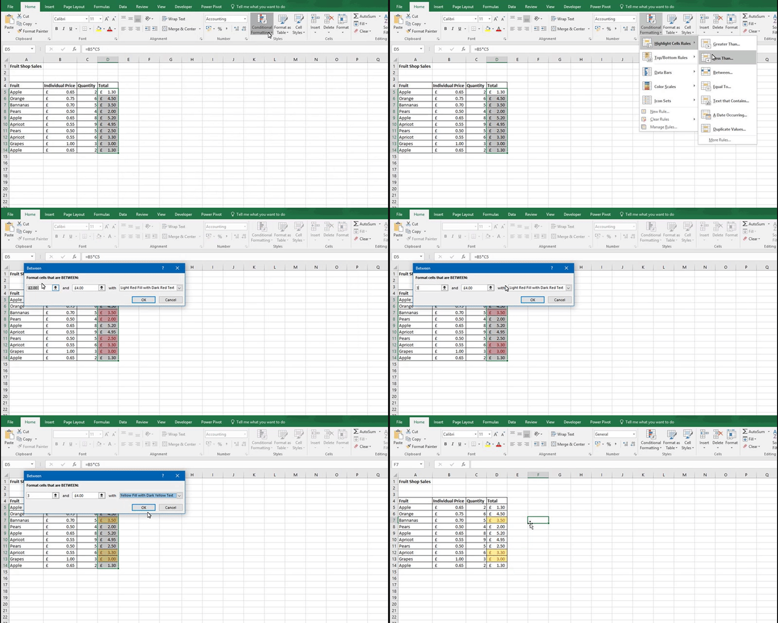
If you want figures that are between two set values to go a certain colour, then use the Conditional Formatting tool. Conditional Formatting allows you to add colour to a spreadsheet based on a condition.
Just go to the Home tab > Conditional Formatting > Highlight Cell Rules > Between.
Type in the figures that are going to be your upper and lower limit, e.g. if you want all numbers between 20 and 40 to be formatted, then type 20 and 40 into the condition boxes.
Finally select a colour that you want the cell(s) to change to.