How to use the AND formula?


If you want to check that multiple conditions in your spreadsheet are TRUE, then we can use the AND formula.


For example, if you wanted to check if a number is greater than 10 but less than 50 we could use an AND formula. The formula in this example would be =AND(A5>10,A5<50)


Another example that you could use the AND formula is to compare two cells to check that they are the same. The formula for this example would be =AND(A5=10,B5=10)


This content is aimed at the Advanced level.   Click here to view our course overview.

How to use the OR Formula?


We can use the OR formula to test multiple conditions. This formula returns TRUE if a condition has been met and FALSE if none of the conditions have been met.


For example, =OR(A5=50,A5=100) will only return TRUE if cell A5 is equal to 50 or 100. It will return FALSE for everything else.


This content is aimed at the Advanced level.   Click here to view our course overview.

How to calculate the average in Excel using data that includes text and numbers?


If you want to calculate the average using data that includes text and numbers, we have to use the AVERAGEA function. This function converts a text value into a number value. The conversions are below.


Value

Conversion

Tree

0

TRUE

1

FALSE

0

10

10


For the data above, the formula would do (0+1+0+10) / 4 = 2.75


This content is aimed at the Intermediate level.   Click here to view our course overview.

How to add figures based on multiple criteria?


If you want to be able add up figures based on multiple criteria, then we can use the SUMIFS formula. 


The Syntax for this formula is:


Sum Range – the range of numerical values you want to add up


Criteria Range 1, Criteria Range 2... – the data ranges that you will find the criteria’s


Criteria 1, Criteria 2... - the items that you want to find in the criteria ranges to be able to calculate the sum.


This content is aimed at the Advanced level.   Click here to view our course overview.

How to count items based on multiple criteria?


If you want to be able to count items based on multiple criteria, then we can use the COUNTIFS formula. 


The Syntax for this formula is:


Criteria Range 1, Criteria Range 2... – the data ranges that you will find the criteria’s


Criteria 1, Criteria 2... - the items that you want count in the criteria ranges


This content is aimed at the Advanced level.   Click here to view our course overview.

How to remove spaces from the beginning and end of a string of text?


In Excel you can use a function called TRIM to remove spaces from the beginning and end of a string of text. 


To use it type =TRIM(  and then insert the cell reference that you want to remove spaces from.


This content is aimed at the Advanced level.   Click here to view our course overview.

How to convert text to uppercase?


In Excel you can convert text to uppercase using the UPPER function.


To use it type =UPPER(  and then reference the cell that you want to convert to uppercase.


This content is aimed at the Advanced level.   Click here to view our course overview.

How to convert text to lowercase?


In Excel you can convert text to lowercase using the LOWER function.


To use it type =LOWER(  and then reference the cell that you want to convert to lowercase.


This content is aimed at the Advanced level.   Click here to view our course overview.

How to capitalise the first letter of each word in a string of text?


If you want to capitalise the first letter in a string of text, then you can use the PROPER function. 


To use this formula type =PROPER(  and then reference the cell that you want to convert.


This content is aimed at the Advanced level.   Click here to view our course overview.

How to extract the middle of a string of text?


If you want to extract the middle part of a string of text, then you can use the MID function.


The syntax for this function is:


Text – the text that you want to extract the middle from


Start Num – the character number of the first character you want to pull data from


Num Chars – the number of characters you want to extract


This content is aimed at the Advanced level.   Click here to view our course overview.

How to count how many characters a string of text has?


If you want Excel to return the amount of characters there are in a string of text then you can use the LEN function. 

To use this formula type =LEN(  and then reference the cell that you want excel to count the characters for. This will then return you with a number that represents how many characters there are in that cell including spaces.


This content is aimed at the Advanced level.   Click here to view our course overview.

How to extract the left side of a string of text?


If you want to extract the left side of a string of text, then you can use the LEFT function.


The syntax for this function is:


Text – the text that you want to extract the left-hand side of text from


Num Chars – the number of characters you want to extract


This content is aimed at the Advanced level.   Click here to view our course overview.

How to extract the right side of a string of text?


If you want to extract the right side of a string of text, then you can use the RIGHT function.


The syntax for this function is:


Text – the text that you want to extract the right-hand side of text from


Num Chars – the number of characters you want to extract


This content is aimed at the Advanced level.   Click here to view our course overview.

How to link sheets in Excel?


Linking sheets in Excel allows you to reference a cell in your formula that is located on a different sheet. 


To do this, start typing your formula and then when you get to the cell you need to reference on another sheet, click on the sheet and then the cell you want to reference. This will now reference that selected cell in your formula.


This content is aimed at the Intermediate level.   Click here to view our course overview.

How to link workbooks in Excel?


Linking workbooks in Excel allows you to reference a cell in your formula that is located on a different workbook. 


To do this, start typing your formula and then when you get to the cell you need to reference on another workbook, click on the workbook, then the sheet and then the cell you want to reference. This will now reference the selected cell from the specified workbook in your formula.


This content is aimed at the Intermediate level.   Click here to view our course overview.

How do I sum values based on a criteria?


If you want to sum values but only for a certain criteria, then we can use the SUMIF formula.


The SUMIF formula consists of three parts which are:


·         Range – the list of data that you want Excel to find the Criteria in


·         Criteria – the item that you want Excel to find in the Range


·         Sum Range – the range of figures that you want Excel to use


So for example, if you wanted to sum up the sales figures for a particular person, your range would be the list of staff names, your criteria would be the staff members name and finally your Sum Range would be the column that contains the sales totals.


This content is aimed at the Intermediate level.   Click here to view our course overview.

How do I count items based on a criteria?


If you want to count how many times an item appears in a range of cells, then we can use the COUNTIF formula.


The COUNTIF formula consists of two parts which are:


·         Range – the list of data that you want Excel to find the Criteria in


·         Criteria – the item that you want Excel to count in the range


So for example, if you wanted to count how many times a persons name appears in a list, your Range would be the list of staff names and the Criteria would be the persons name that you want to count in that list of staff names.


This content is aimed at the Intermediate level.   Click here to view our course overview.

How do I calculate the average based on a criteria?


If you want to calculate the average based on a criteria, then we have to use the AVERAGEIF formula.


The AVERAGEIF formula consists of three parts which are:


·         Range – the list of data that you want Excel to find the Criteria in


·         Criteria – the item that you want Excel to find in the Range


·         Average Range – the figures that you want Excel to use to calculate the Average


So, for example, if you wanted the calculate the average house prices based on the number of bedrooms, your range would be the list of bedrooms each house has got. The criteria would be a specified number of bedrooms and finally your Average Range would be the list of house prices.


This content is aimed at the Intermediate level.   Click here to view our course overview.

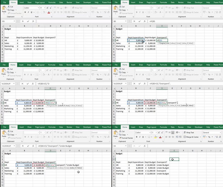
How to create an IF formula


An IF formula is where we give Excel a statement and it will return an answer based on that statement. For example, if expenditure is greater than budget then return overspent, otherwise return under budget.


The Syntax for an IF formula is IF(Logical_Test, Value_if_True, Value_if_False)


The Logical Test is the statement that Excel uses to be able to return the right answer. In the Logical Test we must use Conditional Logic symbols which are > (greater than), < (less than), >= (greater than or equal to), <= (less than or equal to), = (equal to), <> (not equal to).


Value if True is the answer you want Excel to return if the Logical Test is met.


Value if False is the answer you want Excel to return if the Logical Test isn’t met.


For your Value if True and Value if False you can use text (which must be in speech marks), cell references, numbers and formulas.


This content is aimed at the Intermediate level.   Click here to view our course overview.

How to find the largest number in a range of cells


If you want to find the largest number in a range of cells, then use the MAX function. To create this formula type =MAX(

After the open bracket input the range of cells that you want to find the highest value for. To finish close your bracket and press enter.


This content is aimed at the Introduction level.   Click here to view our course overview.

How to find the smallest number in a range of cells


If you want to find the smallest number in a range of cells, then use the MIN function. To create this formula type =MIN(

After the open bracket input the range of cells that you want to find the lowest value for. To finish close your bracket and press enter.


This content is aimed at the Introduction level.   Click here to view our course overview.

How to count cells that contain numbers


If you want to count numbers in a range of cells, then use the COUNT function. To create this formula type =COUNT(

After the open bracket input the range of cells that you want to count. To finish close your bracket and press enter.


This content is aimed at the Introduction level.   Click here to view our course overview.

How to find the numeric representation of a Column


You can use the COLUMN function to return the column number of the cell that you have referenced. For example, column A = 1, B = 2, C = 3 etc.

To use the formula type =COLUMN( and then input the cell that you want to find the column number for. 


This content is aimed at the Introduction level.   Click here to view our course overview.

How to count how many columns there are in an array


You can use the COLUMNS function to count how many columns there are in an array.

To use this function, type =COLUMNS( then select the array of data that you want to count. Finally, close your bracket and press enter for Excel to return your answer.


This content is aimed at the Introduction level.   Click here to view our course overview.

How to find the numeric representation of a Row


You can use the ROW function to return the row number of the cell that you have referenced. For example, row 1 = 1, row 2 = 2, row 3 = 3 etc.

To use the formula type =COLUMN( and then input the cell that you want to find the column number for.


This content is aimed at the Introduction level.   Click here to view our course overview.

How to count how many rows there are in an array


You can use the ROWS function to count how many rows there are in an array.

To use this function, type =ROWS( then select the array of data that you want to count. Finally, close your bracket and press enter for Excel to return your answer.


This content is aimed at the Introduction level.   Click here to view our course overview.

How to create a VLOOKUP


If you are working in columns and want to pull information across from data that can be located either on the same sheet, different sheet or even different workbook, then we can use a VLOOKUP formula.

To create a VLOOKUP formula, click in the cell that you want to pull information to and then type =VLOOKUP( . You will then get a syntax that looks like VLOOKUP(lookup_value, table_array, col_index_num, [range_lookup]).

Lookup Value – the value you want it to look up


Table Array – the data range that you want to find the value in


Col Index Num – the column that you want to extract data from


Range Lookup – True/1 = Approximate - if it can’t find the correct lookup value it will pull across the nearest value that’s less than it.


                    False/0 = Exact – if it can’t find exactly what you’ve asked then it will error


This content is aimed at the Intermediate level.   Click here to view our course overview.

How to create a HLOOKUP


If you are working in rows and want to pull information across from data that can be located either on the same sheet, different sheet or even different workbook, then we can use a HLOOKUP formula.

To create a HLOOKUP formula, click in the cell that you want to pull information to and then type =HLOOKUP( . You will then get a syntax that looks like HLOOKUP(lookup_value, table_array, row_index_num, [range_lookup]).


Lookup Value – the value you want it to look up


Table Array – the data range that you want to find the value in


Row Index Num – the row that you want to extract data from


Range Lookup – True/1 = Approximate - if it can’t find the correct lookup value it will pull across the nearest value that’s less than it.


                    False/0 = Exact – if it can’t find exactly what you’ve asked then it will error


This content is aimed at the Intermediate level.   Click here to view our course overview.

How to stop cells from changing when dragging your formula down


If you’re dragging formulas down using the Autofill tool, then you might notice that the cell references change as well. Sometimes you will want them to change, but sometimes you want the cell references to stay the same. To stop the cell references from changing we must use dollar signs in our formulas.

To stop cell references from changing when dragging down we need to put a dollar sign before the number. For example, if your formula was =B5*H2 and you didn’t want H2 to go to H3, then you would put the dollar sign before the 2. So, your formula would look like =B5*H$2.


This content is aimed at the Introduction level.   Click here to view our course overview.

How to stop cells from changing when dragging your formula across


If you’re dragging formulas across using the Autofill tool, then you might notice that the cell references change as well. Sometimes you will want them to change, but sometimes you want the cell references to stay the same. To stop the cell references from changing we must use dollar signs in our formulas.

To stop cell references from changing when dragging across we need to put a dollar sign before the letter. For example, if your formula was =D4*J2 and you didn’t want J2 to go to K2, then you would put the dollar sign before the J. So, your formula would look like =D4*$J2.


This content is aimed at the Introduction level.   Click here to view our course overview.

How to use the TEXTJOIN function


If you want to join text strings together, then why not try the TEXTJOIN function. This formula also allows you to put a delimiter between each text string. The syntax for this formula is =TEXTJOIN(delimiter, ignore_empty, text1, [text2], …).


Delimiter – the text string that you want to appear between each referenced text string


Ignore Empty – If TRUE, excel will ignore any blank cells


Text 1 – the first string of text you want to reference


Text 2 – the second string of text you want to reference (optional)


This content is aimed at the Advanced level.   Click here to view our course overview.

How to use the TYPE function


If you want to know what data type a value is in a cell, then use the TYPE function. The syntax for this formula is =TYPE(value).

When you have completed the formula, Excel will return a number which represents the data type.

1 = Number

2 = Text

4 = Logical

16 = Error

64 = Array


This content is aimed at the Advanced level.   Click here to view our course overview.

How to use the SEARCH formula?


If you want to search for a string of text within a larger string of text, then use the SEARCH function. This function will return the character number of where the string of text is located. For example, if you wanted to find N in phone, the SEARCH function would return 4 as N is the fourth character along.


The syntax for this formula is =SEARCH(Find Text, Within Text, [Start Number])


Find Text – The text you want Excel to find


Within Text - the string of text you want to find something in


Start Number – the character that you want Excel to start searching from (optional)


This content is aimed at the Advanced level.   Click here to view our course overview.

How to use the FIND formula?


If you want to search for a string of text within a larger string of text, then use the FIND function. This function will return the character number of where the string of text is located. For example, if you wanted to find the letter O in laptop, the FIND function would return 5 as O is the fifth character along.


The syntax for this formula is =FIND(Find Text, Within Text, [Start Number])


Find Text – The text you want Excel to find


Within Text - the string of text you want to find something in


Start Number – the character that you want Excel to start searching from (optional)


This content is aimed at the Advanced level.   Click here to view our course overview.

How to use the CHOOSE formula?


If you want to select an item from a list based on an index number, then why not try the CHOOSE formula. For example, if you had a list of days starting with Monday and you asked excel to return the day that corresponded with index number 3 then excel would return Wednesday.


The syntax for the CHOOSE function is =CHOOSE(index_num, value 1, [value 2],...)


Index Number – the number excel is going to use to find the correct item from the list


Value 1 – the first value on your list


Value 2 – the second value on your list (optional)


This content is aimed at the Advanced level.   Click here to view our course overview.

How to use the SUBSTITUTE function?


If you want to change specific text with new text in a cell, then use the SUBSTITUTE function. The syntax for the SUBSTITUE formula is =SUBSTITUTE(text, old_text, new_text, [instance_num])


Text – the string of text that contains the text that you want to replace 


Old Text – the text that you want to replace


New Text – the text you want to replace the old text with


Instance  Num (Optional) – which occurrence of the old text you want to replace with the new text. If this is not completed excel will replace every occurrence.


This content is aimed at the Advanced level.   Click here to view our course overview.

How to use the ROUNDDOWN function in Excel?


If you want numbers to always round down, then use the ROUNDDOWN function in excel. The Syntax for this formula is =ROUNDDOWN(num, num digits).


Num – the cell that you want to round


Num digits – the number of decimal places you want to round down to, for example 1 would round down to one decimal place


This content is aimed at the Intermediate level.   Click here to view our course overview.

How to check if a value is a number in Excel?


If you want to check if a value is a number, then use the ISNUMBER function. To use it, type in =ISNUMBER( and then the cell you want to reference. When you hit return you will get either a TRUE or False answer. If you get TRUE returned, it means that the value is a number, date or time. Therefore, if you get FALSE returned it means that the value is not a number value.   


This content is aimed at the Intermediate level.   Click here to view our course overview.

How to check if a value is a non-text value in Excel?


If you want to check if a value is a non-text value, then use the ISNONTEXT function. To use it, type in =ISNONTEXT( and then the cell reference you want to check. If you get FALSE returned, it means that the value of the cell is a text value. If you get TRUE returned it means that the value is a numerical value such as a number, date or time. You will also get TRUE returned for a blank cell.


This content is aimed at the Intermediate level.   Click here to view our course overview.

How to find the highest value based on one or multiple criteria?


If you want to find the highest value in a data set based on one or multiple criteria, then use the MAXIFS function. For example, if you wanted to find Dave’s highest sales figure for a product that has a product ID of 1.1 then I would use the MAXIFS function. 


The syntax for the MAXIFS formula is =MAXIFS(max range, criteria range 1, criteria 1, criteria range 2, criteria 2,…)


Max range – the range of cells you want to find the highest value in


Criteria range 1 – the range of cells that you want to find the criteria in


Criteria 1 – the criteria or condition that you want to find the highest value for


Criteria range 2 – the second range of cells that you want to find the second criteria in (Optional)


Criteria 2 – the second criteria or condition that you want to find the highest value for (Optional)


This content is aimed at the Advanced level.   Click here to view our course overview.

How to find the smallest value based on one or multiple criteria?


If you want to find the lowest value in a data set based on one or multiple criteria, then use the MINIFS function. For example, if you wanted to find Dave’s lowest sales figure for a product that has a product ID of 1.1 then I would use the MINIFS function. 


The syntax for the MINIFS formula is =MINIFS(min range, criteria range 1, criteria 1, criteria range 2, criteria 2,…)


Min range – the range of cells you want to find the lowest value in


Criteria range 1 – the range of cells that you want to find the criteria in


Criteria 1 – the criteria or condition that you want to find the lowest value for


Criteria range 2 – the second range of cells that you want to find the second criteria in (Optional)


Criteria 2 – the second criteria or condition that you want to find the lowest value for (Optional)


This content is aimed at the Advanced level.   Click here to view our course overview.

How to check if a value is text in Excel?


If you want to check if a value is text, then use the ISTEXT function. To apply it, type =ISTEXT( and then reference the cell you want to check. When you hit return you will either get a TRUE or FALSE answer. If you get TRUE returned, it means the cell you have referenced is a text value. If FALSE is returned, then you have a numerical value in the cell you referenced, for example, a number, date or time. A blank cell will also return FALSE.


This content is aimed at the Intermediate level.   Click here to view our course overview.

How to use the ROUND function in Excel?


If you want numbers in excel to round up or down to a specified number of decimal places, then use the ROUND function in Excel. The Syntax for the ROUND function is =ROUND(num, num digits). 


Num – the cell that you want to round


Num digits – the number of decimal places you want to round to, for example 2 would round to two decimal places


This content is aimed at the Intermediate level.   Click here to view our course overview.

How to use the ROUNDUP function in Excel?


If you want numbers to always round up, then use the ROUNDUP function in excel. The Syntax for this formula is =ROUNDUP(num, num digits).


Num – the cell that you want to round


Num digits – the number of decimal places you want to roundup to, for example 1 would round up to one decimal place


This content is aimed at the Intermediate level.   Click here to view our course overview.

How to replace text with new text in Excel?


If you want to replace a section of text, then give the REPLACE function a go. This function allows you to replace a specified amount of characters with new text.


The syntax for the REPLACE function is =REPLACE(old text, start num, num chars, new text)


Old text – the text that you want to replace 


Start num – the first character that you want to replace


Num chars – the amount of characters you want to replace


New text – The new text you want to replace the old text with 


This content is aimed at the Advanced level.   Click here to view our course overview.

How to use the COUNTBLANK function?


If you want to count how many blank cells there are in a range, then why not use the COUNTBLANK function.

To use it, type in =COUNTBLANK( and then put in the range of cells that you want it to count the blanks. 


This content is aimed at the Advanced level.   Click here to view our course overview.

What is this week’s number in the current year?


A quick way of finding out which week of the year we are up to is by using the WeekNum function. Once this formula is completed, it will return a number which is based on the week number that you are up to in that current year.

To use the formula, type the function =WeekNum( and then put in a date. Excel will then return the week number that date falls in. If you want it to be dynamic then why not replace the date with the TODAY function.


This content is aimed at the Advanced level.   Click here to view our course overview.

How to find the Median of a range of numbers?


If you want to find the middle value of a range of figures, then use the MEDIAN function in Excel. Type =MEDIAN( and then insert the range of cells you want to find the Median of. When you hit return it will provide you with the median.


This content is aimed at the Intermediate level.   Click here to view our course overview.

How to find the Mode of a range of numbers?


If you want to find which number appears most often in a range of cells, then use the MODE function. In a cell type =MODE( and then insert the range of cells you want to find the mode of. When you hit return it will provide you with the mode.


This content is aimed at the Intermediate level.   Click here to view our course overview.

How to find if a number is odd in excel?


If you need a formula that will return if a number is odd, then why not give the ISODD function ago. Type in the function =ISODD( and then select the cell you want to reference. When you hit enter it will either return a TRUE or FALSE answer. TRUE means the number is odd and false means that it’s an even number. 


This content is aimed at the Intermediate level.   Click here to view our course overview.

How to find if a number is even in excel?


If you need excel to return a number as Even then use the ISEVEN function. Type =ISEVEN( and then select the cell you want to reference. If you get a TRUE answer it means that the number is even. If you get a FALSE answer it means that the number is odd.


This content is aimed at the Intermediate level.   Click here to view our course overview.

Convert pounds to kilograms, meters to yards and teaspoons to tablespoons?


If you struggle with converting data from one unit to another, then why not let Excel’s Convert formula do it for you. 

To use it, type in the function =CONVERT( , type in the number you want to convert, choose the unit you want to convert the number from and then choose the unit you want to convert the number to. 

For example, if I want to see how much 1000g would be in pounds (mass), then I would type =CONVERT(1000,”g”,”lbm”). 


This content is aimed at the Advanced level.   Click here to view our course overview.

How to use Excel to find PI?


If you need to use the value of PI within calculations, but struggle to remember the value of PI, then how about using the PI function in Excel. Just type in =PI() and it will give the value of PI up to 15 digits.

You can then use the PI function to calculate the area of a circle .A=πr2


This content is aimed at the Advanced level.   Click here to view our course overview.

What does it mean if you have a #DIV/0! In a cell?


If you have a #DIV/0! error in your spreadsheet it means that you have a dividing error. A dividing error is caused because the formula is trying to divide by zero. For example, if your formula was =10/0 then it would return a #DIV/0! error.


This content is aimed at the Intermediate level.   Click here to view our course overview.

What does it mean if you have a #REF! In a cell?


The #REF! error appears in a cell if the formula is referenced to cells that cannot be found. This can occur if the referenced cells have been deleted or have been pasted to another location. 


This content is aimed at the Intermediate level.   Click here to view our course overview.

What does it mean if I have #N/A in a cell?


A #N/A error in a spreadsheet means that the formula cannot find what you asked it to look for. For example, in a VLOOKUP formula, if you ask it to look for an ID number that it can’t find, it will return #N/A.


This content is aimed at the Introduction level.   Click here to view our course overview.

What does it mean if I have #NAME? in a cell?


If you see a #Name? error in a cell, then this means there is a typo in the formula. For example, if my formula was =SUM(A5:A), it would return a #NAME? error as the second cell reference is not complete. 


This content is aimed at the Introduction level.   Click here to view our course overview.

What do green triangles in a cell mean


If you see a green triangle in the top left-hand corner of a cell then this means there is some sort of error in that cell such as an inconsistent formula, which is where a formula is different to the other formulas in the surrounding cells, or cells that contain a formula that result in an error. 


This content is aimed at the Introduction level.   Click here to view our course overview.

What does it mean if I have #VALUE! in a cell


If you have got a #VALUE! error in a cell, then there are a couple of potential reasons why. The first is that there is something wrong with the cells you are referencing. For example, if you have a multiplication formula such as =A5*B5, and the value of A5 is a number and the value of B5 is text, then you will get a #VALUE! error as you can’t multiply a number with text.

The other reason you may have a #VALUE! error is because there might be an issue with the way the formula is typed.


This content is aimed at the Introduction level.   Click here to view our course overview.

How to count how many times a value appears in a list?


The Frequency formula counts how many times a value appears in a range. It then places the results into a summary table. The formula does return multiple answers.

Therefore, once you have typed your formula into Excel, instead of pressing Enter, we press Ctrl + Shift + Enter.


This content is aimed at the Intermediate level.   Click here to view our course overview.

How to remove #N/A from a spreadsheet?


If you keep getting #N/A’s in your spreadsheets, then how about forcing Excel to show a different value. To do this we use the IFNA function.

To apply it to your formulas, nest it around the formula just like the image above.


This content is aimed at the Introduction level.   Click here to view our course overview.

How to remove errors from a spreadsheet?


If you keep getting errors in your spreadsheets, then how about forcing Excel to show a different value. To do this we use the IFERROR function.

To apply it to your formulas, nest it around the formula just like the image above.


This content is aimed at the Introduction level.   Click here to view our course overview.

How do I check if a cell is completely empty?


In Excel, you can usually see If a cell is empty. However, sometimes the cell might look empty but in fact it may have a space in it and this can cause problems. To check if your cells are empty, try the ISBLANK formula. Type in the function and the cell reference of the cell you want to check.

If Excel returns the answer TRUE, the cell is empty. If Excel returns FALSE then there is Something in that cell.


This content is aimed at the Introduction level.   Click here to view our course overview.

Find out what the date is after X amount of working days from today?


If you want to work out what the date is in so many working days, then why not try the WORKDAY function.

The WORKDAY function allows you to count so many working days into the future from a specified date. To use it, type the function =WORKDAY(. Then use the Today function for your start date and a number of working days you want to count from that start date. 

It will then give you a number as your answer which you will then need to format into a date. 


This content is aimed at the Advanced level.   Click here to view our course overview.

How do I count cells with text and numbers in them?


You may have come across the Count formula, which counts nonempty cells that contain numbers. Unfortunately, it won’t count cells that have text in them. So instead we use the COUNTA formula. This will count nonempty cells that include text.

So to put it into context, we type in the function and then give Excel the range that we want Excel to count, e.g. =COUNTA(A5:A10).


This content is aimed at the Intermediate level.   Click here to view our course overview.

How to add comments to your formulas?


If you want to add a comment or description to your formulas so you know what they mean, then why not try this tip. After your formula, type +N(“ “). Within the speech marks type your comment. This will leave a comment in your formula without effecting it.  


This content is aimed at the Advanced level.   Click here to view our course overview.

How do I add together the values of multiple columns in Excel?

Excel has a feature called AutoSum. This allows you to add up values quickly.


 How to add multiple columns

1. Select the values that you want to add together and the cells you want the answers to go in.

2. Go to the Home tab, Editing and select AutoSum.


This content is aimed at the Introduction level.   Click here to view our course overview.

How to find the average in Excel?

Excel has a built in option for this, the AVERAGE Function.


How to calculate the average

1. Select the values that you want to find the averages of and the cells you want the answers to go in.

2. Go to the Home tab, Editing and select the AutoSum dropdown.

3. Select Average from the dropdown.


This content is aimed at the Introduction level.   Click here to view our course overview.

How do I find the square root of a number in excel?


If you want to find the square root of a number in Excel, use the SQRT function. 

The formula will be =SQRT(the cell which contains the number you want to find the square root of).


This content is aimed at the Advanced level.   Click here to view our course overview.

How to apply formula placeholders in Excel?


If you want help completing formulas then how about using formula placeholders. All you have to do is type in your function, e.g. =SUM(, then press CTRL + SHIFT + A. This will place the individual parts of your formula into your formula. You can then use the placeholder to help you complete your formula.


This content is aimed at the Advanced level.   Click here to view our course overview.

How to use wildcards in a SUMIF formula?


A SUMIF formula allows you to add up figures in a range that meets specified criteria. For example, if I wanted to add up all the figures in a range for apples, the formula would look like =SUMIF(A:A,”Apples”,D:D). 

If I wanted to add up figures for all fruit beginning with A, i.e Apples and Apricots, I would introduce a wildcard into my criteria. The formula would then be =SUMIF(A:A,”A*”,D:D).

I can also add up figures based on how many letters there are in a string of text. For example, if I want to add up the figures for all fruit that contains six letters, i.e. Grapes and Orange. The formula would be =SUMIF(A:A,”??????”,D:D).


This content is aimed at the Intermediate level.   Click here to view our course overview.

How to use wildcards in a COUNTIF formula?


A COUNTIF formula allows you to count how many times specified criteria appears in a range. For example, if I wanted to count up how many times their was a sale for Apples, the formula would look like =COUNTIF(A:A,”Apples”). 

If I wanted to count how many sales for fruit beginning with A happened, i.e Apples and Apricots, I would introduce a wildcard into my criteria. The formula would then be =COUNTIF(A:A,”A*”).

I can also count based on how many letters there are in a string of text. For example, if I want to count all fruits that contain six letters, i.e. Grapes and Orange. The formula would be =COUNTIF(A:A,”??????”).


This content is aimed at the Intermediate level.   Click here to view our course overview.

How to use wildcards in an AVERAGEIF formula?


An AVERAGEIF formula allows you to find the average based on specified criteria. For example, if I wanted to find the average for apple sales, the formula would look like =AVERAGEIF(A:A,”Apples”,D:D). 

If I wanted to find the average for all fruit beginning with A, i.e Apples and Apricots, I would introduce a wildcard into my criteria. The formula would then be =AVERAGEIF(A:A,”A*”,D:D).

I can also find the average based on how many letters there are in a string of text. For example, if I want to find the average for all fruits that contain six letters, i.e. Grapes and Orange. The formula would be =AVERAGEIF(A:A,”??????”,D:D).


This content is aimed at the Intermediate level.   Click here to view our course overview.

How to find the percentage of a year?


Excel allows you to calculate the percentage of a year based on two dates. All you do is give excel a start date, finish date, Basis (How many days of the year you want to include) and the YEARFRAC formula. 

The formula will then be =YEARFRAC(Start Date, Finish Date, Basis)

It will give the answer as a decimal, but you can quickly format it to a percentage by going to the Home tab > Number group and select the percentage icon.


This content is aimed at the Advanced level.   Click here to view our course overview.

How to generate random numbers in Excel?


If you want to generate a random number in Excel, you have a couple of options. The first is using the RAND function. Just type =RAND() into Excel and it will give you a random number between 0 and 1.

If you want a random whole number between a specified range, then use the formula RANDBETWEEN. So for example, if I want to generate a random whole number between 1 and 20, my formula would be =RANDBETWEEN(1,20). 


This content is aimed at the Intermediate level.   Click here to view our course overview.